We explore the star-triangle relation in statistical mechanics and see how, through knot theory it can connect to a multitude of other, exactly solvable systems in physics

Back to homepage https://principiaphysicaegeneralis.com/

Introduction

Exactly solvable problems in physics are far and few in between. Whether it’s statistical physics or quantum mechanics, most of the physically important systems are treated either perturbatively or numerically. Both of these methods are approximations of the real solution, they sometimes miss important properties and they always miss the mathematical satisfaction of an exact solution.

Although rare, in the last 30 years there has been growing work on exactly solvable (or from now on integrable) systems and in particular systematising them. This systematisation comes in the form of the Yang-Baxter equations we will encounter in this article, equations which connect all sorts of integrable systems through the language of knots and braids. This is an on going field of research and so this article will only attempt to scrape the very top of these ideas, hopefully without losing all of the beauty in the process.

In the first chapter we will see how an equivalence called the star-triangle relation was originally discovered and used to solve the Ising model in 2 dimensions and how it can be generalised. In the second chapter we will see how the star-triangle relation can be translated into the language of knots and braids. Then, in the third chapter we will see how this correspondence can connect even more integrable problems in both statistical physics and quantum mechanics.

The star-triangle relation

The generals of a statistical system

We begin our journey by studying one of the simplest statistical systems, the Ising model. This model is composed of a lattice in \(d\) dimensions, that means a collection of points (vertices) connected by edges. At each vertex we will place a spin (for example electrons orbiting nuclei) that can be either pointing up or down. Lastly we will assume that the spins interact with their nearest neighbours. The resulting system can be characterised by the energy per vertex. It is given by $$ E_i = \sum_j Js_is_j + Hs_i, \;\;s_i=\pm 1\;\;\; (1.1) $$ Where \(j\) is summed over all of the nearest neighbours of the i-th spin, \(J\) is a constant and \(H\) is the external magnetic field we can apply.

What we mean by solving a system is that we find the form of its partition function \(Z\) defined as $$Z = \sum_s e^{-E/kT} \;\;\; (1.2)$$ where we sum over all possible states \(s\) of the system as a whole and \(E=\sum_i^N E_i\) the total energy of the system. \(T\) is the temperature of the system and \(k\) is Boltzmann’s constant. Often we will write the above equation as $$Z = \sum_s\prod_i w_i $$ where \(w_i = e^{E_i/kT} \) is called the Boltzmann weight of vertex \(i\).

Having computed the partition function we can get all physically relevant quantities we would ever need from the system’s free energy \(F\) $$ F(H,T) = \lim_{N\rightarrow \infty} kT\log(N^{-1}Z) \;\;\; (1.3) $$ N is the number of vertices and the limit we take is called the thermodynamic limit. For example, the system’s magnetisation is given by \(M=-\frac{\partial}{\partial H}F\).

The Ising model was first proposed and solved in one dimension by Ising in 1925. The real breakthrough came in 1944 when the mathematician Onsager solved the same problem on a two-dimensional square lattice. Onsager’s solution was the first of its kind and still inspires many solutions of similar systems. In the introduction to that paper Onsager described in words a “rather obvious” star-triangle transformation that would prove much more important to the advancement of integrable systems than Onsager could imagine.

The star-triangle transformation

The transformation we are about to describe connects an Ising model οn a hexagonal (or honeycomb) lattice to a different Ising model on a triangular lattice. Since, in the end, we sum over all of the possible states of each vertex, we can first integrate the middle vertex of each “star” to get an effective coupling between the outer vertices. Schematically we have

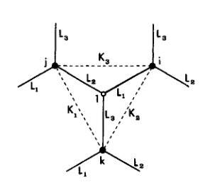Figure 1: The star-triangle transformation from a star on the honeycomb lattice to the dotted triangle

To be more precise, by integrating the white vertex labelled l we go from a “star” of \(L_i\) couplings to a triangle of \(K_i\) couplings. The \(K\)’s are fully determined from the \(L\)’s through quite complex relations like $$ 2\cosh(L_1+L_2+L_3) = R\exp(K_1+K_2+K_3) $$ and so on. In order to make use of this relation and to abstract away from the specific problem it will prove very useful to switch over to the language of operators (or just matrices if operators seem scary). These operators act on the partition function Z to give a different one.

To begin with our system consists of a row of \(N\) spins \(\sigma_i\) and our aim will be to build up the lattice by adding edges and vertices. To that effect we first define the operator \(c_i\) that flips the \(i\)-th spin (if it’s value is \(+1\) is goes to \(-1\) and vice versa). Now we can define the building operators $$ P_i(K)= e^{K\sigma_i\sigma_{i+1}},\;\;Q_i{L} = Q_i(L)=e^L \mathcal{I} + e^{-L}c_i \;\;\;(1.4)$$ where \(\mathcal{I}\) is the identity operator. The operator \(P_i(K)\) adds and edge of strength \(K\) between spins \(i\) and \(i+1\). \(Q_i(L)\) adds a new vertex that is connected to the \(i-th\) vertex by a new edge of strength \(L\). We can think of \(Q_i\)’s new vertex as being above of below spin \(i\) in the row of existing spins. With these two operators we can build any lattice we want step by step (for those who want more of the mathematical details, this part is taken from Baxter’s book on Exactly solved models in statistical mechanics that is also listed in the sources). To make the connection with the star triangle relation we define the diagonal construction operators \(U_i\) as

$$ U_i= \begin{matrix}{ll} P_j(K), & i=2j \\ (2\sinh2L)^{1/2}Q_j(L), & i=2j-1 \\ \end{matrix} $$

This operator creates a “staircase” of spins and it’s enough to construct the square lattice. Going back to the honeycomb lattice we find that the relation in figure 1 can be translated into $$U_{i+1}(K_1,L_1)U_{i}(K_2,L_2)U_{i+1}(K_3,L_3) = U_{i}(K_3,L_3)U_{i+1}(K_2,L_2)U_{i}(K_1,L_1)\;\;\; (1.5) $$ We can write this relation and another property of these matrices more compactly as

$$U_{i+1}U_{i}'U_{i+1}’’ = U_{i}''U_{i+1}'U_{i}\;\;\; (1.6a) $$ $$U_iU_j'=U_j'U_i,\;\; for\;\;|i-j|\geq 2\;\;\; (1.6b) $$

The above relations, and especially (1.6a) will be the “glue” that holds integrable systems together. It is called the Yang-Baxter Equation and we will see in chapter 3 that statistical systems that satisfy it are exactly solvable. But first, we will look at a completely different area of mathematics where a similar relation appears.

Knots and Braids

The theory of knots in mathematics is relatively new (if the 20th century is considered recent) and at first glance it has nothing to do with statistical physics or for that fact anything more abstract than a noose for holding horses outside of saloons. However, as we dive into the mathematical formalism of knots, links and braids we will see how they can tie many different integrable systems together with a common language.

knots, links and graphs

What is a knot anyways? Knots usually have loose ends that we can then tie to other things. To treat them mathematically however we will define a knot as a single closed loop and a link as a composition of many different knots. Typical links are seen below

Figure 2: Simple knots, the first one from the left is the unknot and the second one is known as the trefoil

The unknot is simply a circle that doesn’t overlap with itself. Two knots are topologically the same (or isotopic) if we can continually deform one into the other. This means no cuts, gluings or creation of sharp edges. If a knot can be untied then it is isotopic to the unknot. Reidemeister proved that there are only 3 moves that one needs to do (multiple times if needed) to prove that two links are isotopic. In other words, two links are isotopic if and only if one can be transformed into the other using only the Reidemeister moves below

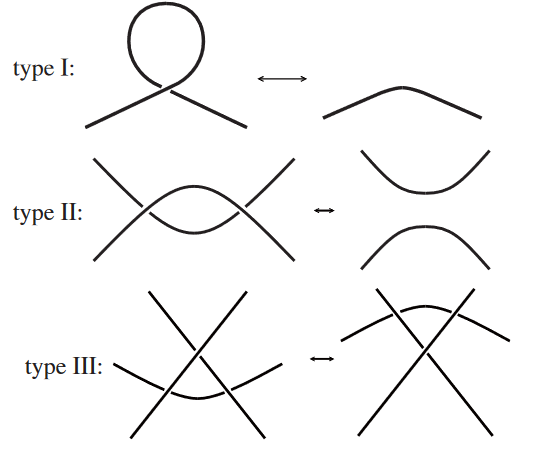
Therefore, if we can define a quantity on a knot that stays the same after the application of the above moves, then we have found a knot invariant, it will take the same value on every isotopic knot.

At first glance knot invariants seem like they belong purely to the domain of mathematics. In fact there are dozens of so-called knot polynomials that mathematicians keep constructing to this day. We will see that with a small change of perspective, a lot of physically relevant quantities in different systems end up being knot invariants.

To make a connection with the last chapter we can turn any link into a graph. It can be proved that any link can be coloured in black and white so that the unbounded “outside” is white and every area only borders areas of a different colour. To make a graph we assign a vertex to each black area and an edge to each link crossing that connects different black areas, for example

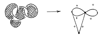
In addition, we can assign a sign to each edge (corresponding for example to the alignment of spins at each vertex), by the type of crossing. The rule goes as follows: imagine you are travelling along the edge and towards a crossing, if the part of the link that sits below the other is to your right then we assign \(+\), otherwise we assign \(-\). Then the type III Reidemeister move can be translated into a relation between graphs

We can already see the similarities between the type III move and the star-triangle relation we saw in Figure 1. To put the correspondence in steadier mathematical footing we will need to turn to the adjacent mathematical field of braids.

Braids and the Yang-Baxter equation

A braid is a set of “strings” that move vertically and can cross over and under one-another. We can define the braid group of N braids \(B_N\) comprised of the elements \(\sigma_i\) (not to be confused with spins). \(\sigma_i\) corresponds to crossing the \(i\)-th strand over the \((i+1)\)-th one. For example, if we have 4 strands then

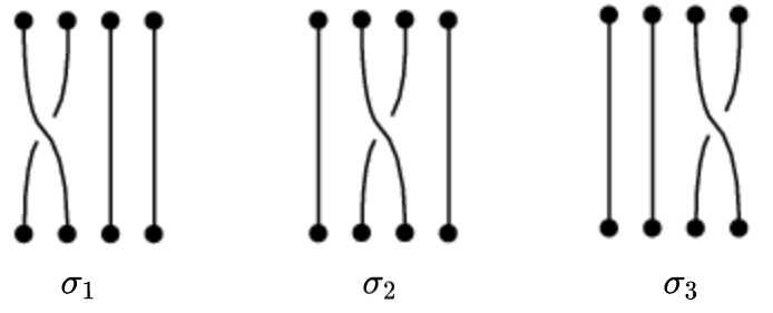
For the above to form a group we also need to define the inverse transformations \(\sigma^{-1}_i\) that correspond to to the opposite move (passing the \(i\)-th strand under the \((i+1)\)-th). Any braid can be constructed by consecutive applications of the generators. The result of “multiplying” two generators can be thought of as applying the second generator to the end points of the first. The braid group is characterised by two properties $$\sigma_{i+1}\sigma_{i}\sigma_{i+1} = \sigma_{i}\sigma_{i+1}\sigma_{i}\;\;\; (2.1a)$$ $$\sigma_{i}\sigma_{j}=\sigma_{j}\sigma_{i},\;\;|i-j|\geq 2\;\;\;(2.1b)$$ Property (2.1a) corresponds to a type III move as can be checked out on paper (The type II Reidemeister move translates into the definitional fact that \(\sigma^{-1}_i\sigma_i =1\)). The observant reader will notice that the group properties (2.1) are exactly the same as the operator relations (1.6) that appeared in the Ising model. This means that the construction operators we defined there form a representation of the braid group and every lattice system can be thought of as a braid.

The last and easiest step of this connection is that between braids and knots. It has been proved that any knot can be represented as a closed braid, that is a braid where all the strands are connected in a loop as seen in the below figure

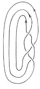
What this means is that any object that satisfies the Yang-Baxter equation (1.6a) is a representation of the braid group and can be mapped onto a knot or a link. This also means that any quantity that is constructed by such objects will be a knot invariant since it doesn’t change under Reidemeister’s moves. In the next chapter we will see how these objects arise in physics

Solving systems with knot invariants

Transfer Matrices

To apply the ideas of knot theory to statistical systems we first need to introduce a tool called the transfer matrix. To do this we will start with the simplest possible system, the Ising model in one dimension. The energy of the system is given by (1.1) where we assume \(i=1,…,N\). To make our life easier we define cyclic boundary conditions so that \(s_{N+1}=s_1\). In the thermodynamic limit where \(N\rightarrow \infty\) the boundary conditions should not affect the system since the boundary is an infinitely small part of the system.

We can now write the partition function (1.2) in the following form (from now on \(kT = 1\)) $$Z_N = \sum_s V(s_1,s_2)V(s_2,s_3)…V(s_N,s_1) \;\;\; (3.1) $$ where $$V(s,s’) = e^{Jss’ + H(s+s’)/2} \;\;\; (3.2) $$ We can think of these as a part of a \(2\times 2\) matrix called the transfer matrix \(V\) $$V = \begin{pmatrix} V(+,+) & V(+,-) \\ V(-,+) & V(-,-) \end{pmatrix} = \begin{pmatrix} e^{J+H} & e^{-J} \\ e^{-J} & e^{J-H} \end{pmatrix} \;\;\; (3.3) $$ then, taking into account the fact that we sum over all possible spins and that the first and last spin in (4.1) are the same, we can write $$Z_N = TrV^N=\lambda^N_1+\lambda^N_2 $$ where the \(\lambda\)s stand for \(V\)’s eigenvalues. Let’s say that \(\lambda_1\) is the biggest eigenvalue, then in the thermodynamic limit we get $$ Z_N \rightarrow \lambda^N_1 $$ and the free energy is $$ F=N^{-1}logZ_N=log\lambda_1 = log(e^j\cosh H +\sqrt{e^{2J}\sinh^2H+e^{-2J}}) \;\;\;(3.4)$$

What we can take from this is that if we know the biggest eigenvalue of the transfer matrix then we can exactly solve the system in question. This is by far the most common way of solving any statistical system. However, in two dimensions each \(V\) corresponds to a whole row of spins and so the possible arrangements, and corresponding elements of the matrix, are \(2^N\), where N is the number of rows. We can see how finding the eigenvalues becomes exponentially harder.

Spin models as Knot Polynomials

If we recall the operators we defined in the first chapter we can see that we can write the transfer matrix in 2 dimensions by repeatedly using \(U_i\) $$V(K,L)=U_1(K,L)…U_n(K,L),\;\;n=2N-1$$ That is, we construct each diagonal row one vertex at a time.

Already we can see that the building blocks of our theory satisfy the braid group relations (1.6) and therefore are unchanged under the Reidemeister moves. This means that the quantity $$ Z_L = \left(\frac{1}{\sqrt{j}}\right)^{V-1} Z_N \;\;\; (3.5) $$ where \(V\) is the number of vertices and \(j\) the number of values than \(s_i\) can take, is a knot invariant. The extra factor is there because, as we can see from Figure 5, after we apply a type III move, we add one vertex to our link or lattice¹.

We can take this a step further thanks to Baxter. If we define \(V=V(L_1,K_1)\) and \(V’=V(L_2,K_2)\) then the Yang-Baxter equation (1.6a) implies that $$VV’=V’V\;\;\; (3.6)$$ This fact, together with some simple assumptions about our system, is enough to find the eigenvalues of \(V\) and so solve the system (see Baxter’s book in the sources). What this means is that any solution to the Yang-Baxter equation (1.6a) can both construct an integrable spin model as well as a knot polynomial.

Vertex Models as Knot Polynomials

There is another type of statistical model that is closely related to spin models. Vertex models are characterised by a set of vertex states that each vertex can take. For example in an ice-type model each vertex corresponds to an atom surrounded by four ions. Two of the ions must be close to the atom while the other two must be at a distance. We then have 6 possible vertices

It is now even easier to project our model onto a knot or link where each strand leaving a crossing is labelled by the corresponding state (ion close to or at a distance from the atom). Indeed we can assign to each vertex a Boltzmann weight based on the state of the four edges connecting to it. For example, labelling the vertices counter-clockwise and starting from the left one, the first vertex of Figure 8 corresponds to \(w(+,+,-,-)\) where \(-\) corresponds to the ion being far away and \(+\) to being close.

It turns out that the weights of this model satisfy the following equation

$$ \sum_{\gamma,\mu’’,\nu’’} w(\mu,a,\gamma,\mu’’)w’(\nu,\gamma,\beta,\nu’’)w’’(\nu’’,\mu’’,\nu’,\mu’)=$$ $$ =\sum_{\gamma,\mu’’,\nu’’} w(\nu,\mu,\nu’’,\mu’’)w’(\mu’’,a,\gamma,\mu’)w’’(\nu’’,\gamma,\beta,\nu’) $$

or in pictorial form:

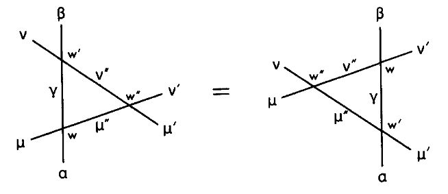
The connection to knots is even more obvious now since this is simply a type III Reidemeister move (see Figure 3). The result is again a general one: Following the exact same steps and as in a spin model, a solution to the Yang-Baxter equation corresponds to an integrable vertex model, the partition function of which is also a knot invariant.

Scattering in Quantum Field Theories as Knot Polynomials

The final model we shall look at is that of quantum particles scattering. In quantum mechanics (and in field theory) the end goal is to calculate probability amplitudes for events to take place.

If a system is described by a set of states \(\ket{n}\), where \(n\) are the quantum numbers (e.g. angular momentum) that define the state, then the probability amplitude of going from state \(\ket{i}\) to \(\ket{f}\) after time T is given by $$ p_{i\rightarrow f} = \bra{f}e^{iHT}\ket{i} \;\;\; (3.7) $$

² where H is the Hamiltonian of the system, similar to the energy (1.1) of a statistical system. In the case of free particles scattering of each other, like in accelerators, the probability amplitude is determined by a quantity called the S-matrix in which case

$$P(k\rightarrow p) = |\bra{p}S\ket{k}|^2$$

where \(p\) and \(k\) are now momenta. The S is just a different name for the operator \(e^{iHT}\) when \(T\rightarrow \infty\) because we assume that the state of the particle(s) was \(\ket{k}\) in the infinite past and \(\ket{p}\) an infinite time after the scattering, so that we can consider both states free (not interacting). Although we won’t calculate them here, the two-particle S-matrix of a theory is the bread and butter of Quantum Field Theories. That is, it is straight forward to calculate probability amplitudes for two particles “colliding” elastically. That is not the case for multi-particle scattering where the computations become substantially more complicated and challenging.

There are however cases where any multi-particle scattering can be viewed like a series of two-particle collisions in sequence. Then the S-matrix is said to be factorisable and the theory is, in a sense solvable for any number of particles. For example the S-matrix of 3 particles in a factorisable theory can be factorised as follows $$S_{3p}=S_{12}(\theta_{12})S_{13}(\theta_{13})S_{13}(\theta_{23}) \;\;\; (3.8) $$

Here \(S_{ij}\) is the S-matrix between particles i and j and \(\theta_{ij}\) is the relative rapidity of the two particles. Rapidity is defined as \(\theta_{ij}=\tanh p_{ij}\) where \(p_{ij}\) the relative momentum.

The important question then, is, when is an S-matrix factorisable? The answer comes in a very familiar form. We make two simple assumptions, the number of particles stays the same after every two-particle collision and the momenta before and after the scattering are the same thanks to the conservation of momentum. These two constraints (in 1+1 spacetime dimensions) lead to the following picture: There are two distinct ways of scattering 3 particles in pairs of two that should give the exact same result, since momentum and particles are conserved. These are the following (where the x axis is space and the y axis time):

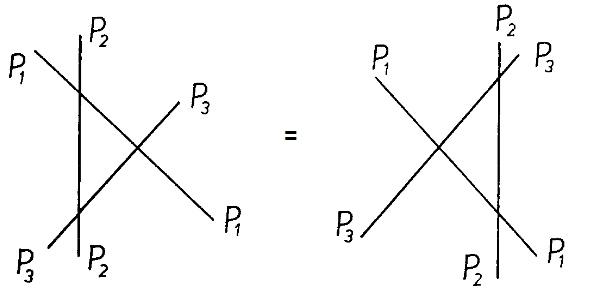
Well, by now we are familiar with the above diagram, it’s a type III Reidemeister move. Written out, we have $$ S_{23}(\theta - \theta’)S_{13}(\theta)S_{12}(\theta’) = S_12(\theta’)S_{13}(\theta)S_{23}(\theta -\theta) \;\;\; (3.9) $$ which as we should expect by now is another form of the Yang-Baxter equation (1.6a). We also have the self evident relation $$ S_{12}(\theta)S_{21}(-\theta)=I_{12}\;\;\; (3.10) $$ where \(I_{12}\) is the identity i.e. nothing happens. This is again an obvious restatement of a type II Reidemeister move.

From the above we can conclude that in \(1+1\) dimensional quantum systems, every factorisable system is also a representation of the braid group and its S-matrix is a knot invariant.

Conclusion and Resources

What started out as an interesting transformation on a 2d lattice spin problem grew into a web of interconnected integrable systems through the language of knots and braids. What we have found is that if a quantity satisfies the Yang-Baxter equation (1.6a) then it corresponds to both a knot invariant and an exactly solvable problem in physics, be that spin models, lattice models or quantum mechanics. This is very interesting and useful both for mathematicians as well as physicists. A mathematician can get a knot invariant from a physicist’s solved system and a physicist can get a solution to a system from a mathematician’s knot invariant.

In the last 30 years there has been a lot of work in systematically finding solutions to the Yang-Baxter equations. The modern approach is a method called Quantum-Groups which involve a lot of high-end mathematical concepts such as Hopf algebras and group deformations. We did not even attempt to scrape the surface of these subjects here.

Back to homepage https://principiaphysicaegeneralis.com/

Resources

[1] Onsager’s original solution of the 2d Ising model and the birth of the star-triangle transformation in statistical mechanics is found in his paper “Crystal Statistics. I. A Two-Dimensional Model with an Order-Disorder Transition” (1944)

[2] A deep exploration of the star-triangle relation as well as integrable statistical systems in general can be found in Baxter’s book “Exactly solved models in statistical mechanics” (1990)

[3] Jones did a lot of pioneering work on the connection between the Yang-Baxter equation, knot invariants and braids. An early review on the subject is his article “On knot invariants related to some statistical mechanical models” (1989)

[4] An interesting and beautifully drawn book, that is however quite (self-admittedly) rambling, is Kauffman’s “Knots and Physics” (2013)

[5] The Yang-Baxter equation first appeared in the context of quantum systems in Yang’s article “Some Exact Results for the Many-Body Problem in one Dimension with Repulsive Delta-Function Interaction” (1967)

[6] The concept was expanded into factorisable quantum field theories by Zamolodchikov and Zamolodchikov in “Factorized S-matrices in two dimensions as the exact solutions of certain relativistic quantum field theory models” (1979)